The projective, or pinhole camera model is the basis for our view on how image formation works for modern cameras. The idea is to construct a mathematical model which maps the three dimensional world into pixels in a two dimensional image. There are many sources, both online and in books, which cover the subject, but I’ve found that many of them are overly theoretical, while others leave out important details necessary for solving real problems. If you would like graduate-level references on projective geometry and image formation, I recommend “Computer Vision: Algorithms and Applications” by Szeliski and “Multiple view geometry in computer vision” by Hartley and Zisserman. What I’ll do here is assume only a basic knowledge of geometry and linear algebra, and try to build from the fundamentals to the full camera model, ending with a real example of monocular pose estimation. Also, I apologize in advance for the poor quality of my diagrams and occasionally abused notation.

The way that the world gets captured as an image can be thought of as happening in three steps:

• First, we need to transform points in the world so that they can be described from the camera’s point of view
• Second, we need to take the points in the camera’s point of view and project them from three dimensions into two dimensions, onto our image plane
• Finally, the two dimensional points in our image plane need to be scaled into pixel units

In this blog, we will deal with the first step, and cover the next two in upcoming blogs, ending with a discussion of the finer points of the full model, and a worked-out example of pose estimation. Of course, projective transformation isn’t the only aspect of image formation – there’s also lighting, material properties, lens optics, semiconductor physics and photochemistry for sensors, and color science for how color is generated and how human eyes perceive color. Perhaps I’ll try to cover some of those topics in future blogs, but for now, let’s get started with part 1.

Part 1: Transformation

Rigid transformations in two dimensions

Instead of starting with three dimensions, it’s instructive to examine rigid transformations (also known as Euclidian transformations) in two dimensions, which contains all of the essential features of 3D, but with less complexity. Here, rigid just means that distance is preserved between points under the transformation, or to put it another way, objects don’t deform under rigid transformations. Let’s start with a few simple examples to get ourselves thinking about how cameras see the world. Imagine a two dimensional world, with a point in its coordinate system written as . A two dimensional camera resides in this world, with its own reference coordinate system glued to itself, with a point it its coordinate system written as . In the diagram below, for example, the camera is sitting a few units away from the origin of the world coordinate system. Units will matter later, but let’s ignore them for now.

We want to ask ourselves how a point described in the world coordinate system, for example , can be described in the camera coordinate system. In other words, how does the world look from the perspective of the camera, or what does the camera see? In this case, it’s easy. The world sees the point one unit to its right, and the camera sees the point four units to its right. This transformation can be written mathematically as

Three things are important to note from this simple example. First, the above equations are a valid mapping from world coordinates to camera coordinates for any world point. Second, we can think of the transformation in multiple ways: as acting on the point, or as acting on the axes. In other words, we can either think about this mapping as translating the point right by 3 units, or as translating the world axes left by 3 units. How you’d like to think about it is up to you – each way can be convenient at different times. Having multiple coordinate systems, and also having no “master” coordinate system to which everything else is relative, might seem strange or complicated at first. However, it’s quite a natural way of looking a the world: if I describe an object as being one meter to my left, and you describe it as four meters to your left, both statements a true if you’re standing three meters to my right!

Next, let’s look at a case where the camera coordinate system is rotated 45 degrees clockwise relative to the world coordinate system:

Again, we want to ask how the point can be described in the camera coordinate system. In this case, the transformation is

This is a little more complcated than the translation case, but is effectively the same sort of thing – the camera points are some linear function of the world points. Under this transformation, the point becomes , so the distance from the origin hasn’t changed. This is what we would expect from a pure rotation. Also, as before, this transformation can be viewed two ways, either as rotating the point 45 degrees counterclockwise, or rotating the world axes 45 degrees clockwise. A convenient way of representing rotation is by using the notation of matrix multiplication. In matrix notation, rotation of a point by is represented as

Composing transformations

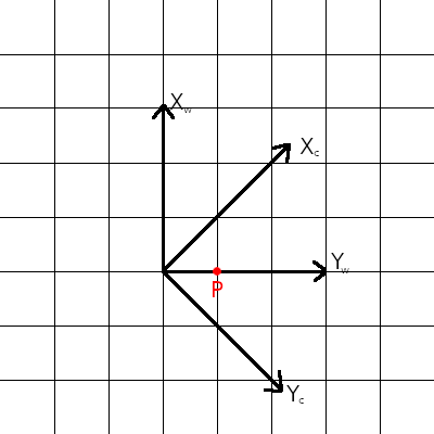
In two (and three) dimensions, the most general rigid transformation is one which involves composing a rotation and a translation – the camera can be anywhere in the world, pointing in any direction! For example, the diagram below shows a situation where the camera is both translated and rotated relative to the world axes:

Before doing any math, let’s do some manual measurement. We can see that in camera coordinates, the point can be reached by moving along the X direction three and a half corner-to-corner distances, and along the Y direction half a corner-to-corner distance. Corner-to-corner distance is , which puts P at in camera coordinates (you should try to calculate this yourself from the picture), so this is the result we should expect after applying our transformation.

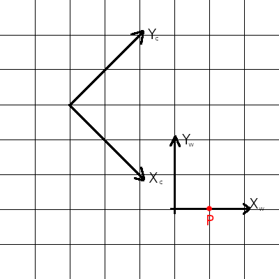
Let’s rotate first, and then translate. We first rotate the point by 45 degrees counterclockwise, and then translate it along the x direction by . Equivalently, we can think of this as rotating the world axes clockwise by 45 degrees, and then translating it along its new x axis by (this might be easier to visualize). This transformation can be written

We can check that this transformation, applied to the point , results in the same answer as the one we computed earlier (recall that is the same as ). An important note here: rotations and transformations are not commutative, which means that, in general, applying a rotation followed by a translation is not the same as applying the same translation followed by the same rotation (the reader is encouraged to show this using the above example). Because of the notation we are about to introduce, the most common way to compose a rotation with a translation is to rotate first, and then translate, though the opposite would still be valid, just with different parameters.

Whereas we were able to represent rotation using the notation of matrix multiplication, we hit a snag when trying to do the same with the equations for the composed transformation because of the term. In order to allow our composed transformation to be represented as a matrix multiplication, we augment the world point with an additional 1, so that our system of equations becomes

or, for a general rotation-followed-by-translation,

One can check that, upon performing the matrix multiplication, one obtains the same equations as before. The way I’ve written the equation here, only one matrix multiplication could be performed before you can no longer multiply the result by a 2x3 matrix. However, we could similarly augment the camera coordinates and add a row to the bottom row of the transformation matrix to allow us to apply any number of transformations in sequence. The reason I didn’t add the extra row is because having the camera coordinates without an extra 1 makes the projection step smoother, and any sequence of rigid transformations (that is, any number of rotations or translations) can be composed into a single transformation matrix, so we don’t lose any generality.

Three dimensional transformations

Scaling up from two to three dimensions is fairly straighforward. We simply add a Z dimension to the world and camera coordinates:

where I’ve written the 3 by 3 rotation part of the matrix using instead of explicitly as a function of angles. Though there are nine elements in the 3D rotation matrix, due to the constraints on how rotation matrices must operate on points, there are only three degrees of freedom, like there was only one in the two dimensional rotation matrix. There are also multiple ways to compose this rotation matrix from rotations about the X, Y, and Z axes, but I won’t try to cover all of this detail here. For interested readers, the Wikipedia article might be a good place to start. In total, there are six degrees of freedom (three rotation, three translation) in the three dimensional transformation matrix. It’s also worth noting that, while I’ve written the transformation matrix as a 3x4 matrix, it’s sometimes written as a 4x4 matrix by adding a bottom row with three zeros and a one.

The 3D transformation matrix is usually referred to as the “camera extrinsic matrix”, and sometimes given the symbol . It’s also sometimes condensed into

or

where is the 3x3 rotation matrix, is the 3x1 translation vector, and is a 1x3 matrix of zeros. Like in the two dimensional case, this transformation matrix maps points in the world coordinate system to the camera coordinate system, as shown in the figure below.

We haven’t worried about any specific locations or orientations for the camera or world coordinates in this blog, except when we made a vague and unuseful statement that the camera axes are glued to the camera somehow. We will leave specifics to the next blog where we define the geometry of the camera. The other question of how to define world coordinates is a practical consideration, and worth some discussion. Do we align the world coordinate system to a corner of the room we’re in, for example? In other words, which transformation are we actually computing? In general, except in special circumstances where there are, perhaps, multiple objects of interest with known locations, making it sensible to have some fixed world coordinate system, it’s best to align the world coordinate system to the object being viewed. This is simply because we usually know more about the structure an object than about the object’s position in the wider world. It’s easier to define a point on a chair relative to the bottom of the chair, rather than relative to the center of the earth, for instance. When we define the world coordinates this way, the transformation matrix tells us how the object is located and oriented relative to the camera, and vice versa, which, as we will see, is useful information. In the more general case where perhaps there is no specific object being viewed, the transformation matrix tells us how the world is oriented relative to the camera, and vice versa. In either scenario, with everything being relative, the transformation matrix provides us with the pose of the camera relative to the world.

It’s important to remember that the values in the transformation matrix change depending on how the geometry is defined, but every definition is a different way of representing the same transform.

Closing remarks

At this point, we’ve covered the mathematics necessary to see the three dimensional world from the camera’s perspective, by transforming world coordinates into the camera’s frame of reference. In the next part, we’ll use this description of the world from the camera’s point of view to bring that 3D world onto the camera sensor in order to create a two dimensional image. This will be where we look at homogeneous coordinates, pinholes, focal lengths, and all of that fun stuff. Stay tuned!

Part 1: Transformation - You’re already here!

Part 2: Projection - here

Part 3: Scaling - here