In the last blog, we covered the first step needed in order to build the projective camera model, rigid transformations in three dimensions. When we last left off, we had written coordinates in the world from the perspective of a set of axes glued to the camera, as $[X_c, Y_c, Z_c]^T$ , but the exact position and orientation of the camera axes were arbitrary. In this blog, we will see how we can transform objects in three dimensions into two dimensional projections on an image, and be specific about the camera’s geometry.

Part 2: Projection

Pinhole cameras

Before we get into any geometry, let’s talk about the pinhole camera, shown below in a figure stolen shamelessly from Wikipedia.

A pinhole camera is a simple camera with a tiny hole in place of a lens. The hole acts as an aperture, creating an inverted image on a flat film surface behind the pinhole. Its operating principle is straightforward:

The pinhole only allows (ideally) only a single ray of light between each visible point in the world and a corresponding point on the film. In other words, one can only draw one line between each point on the film and the pinhole.
When viewed from behind the film (facing the pinhole), the image created by a pinhole camera is inverted in both directions (up-down and left-right).
Because only one ray of light reaches each point on the film, the image created by the pinhole appears clear, or in focus.
If one were to make the hole larger, more than one light ray would be able to reach each point on the film, making the image increasingly blurry, or out of focus.
Making the hole larger also lets more light in, resulting in a brighter image. The relationship between amount of light captured and focus is a fundamental trade-off in vision.

In modern times, true pinhole cameras have largely been relegated to the realm of hobbyists, because lenses eliminate the main drawback of pinholes: with a lens, one can have in-focus images with large apertures by using optics to bend light.

The dominant model for the behavior of cameras, however, still uses a pinhole camera geometry (after a fashion), because it retains all of the geometrical features necessary for computing image projection, without the complexity of modeling the lens. I’m glossing over the entire field of optics with my previous statement, but it’s impossible to cover everything in a single blog post. For the purposes of the pinhole camera model, one can think of the lens as an ideal pinhole which magically allows more light to enter – this is good enough for us, since the amount of light impacting the film doesn’t affect the mathematics of projection.

The pinhole camera model

Like in the first blog, we will look at a two-dimensional version of the camera model. This retains the essential features of the three-dimensional model, without forcing me to spend days drawing a 3D diagram in MS Paint.

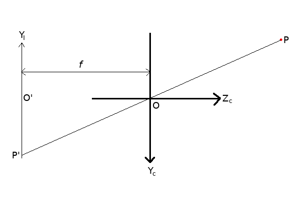
In the figure above, the camera’s pinhole is at the origin, labeled $O$ . The camera’s Y axis points down, and its Z axis points to the right (the X axis, if it were drawn, would point out of the screen). A world point $P(Y_c, Z_c)$ is viewed through the pinhole at $O$ , and light from $P$ strikes the film at $P'$ . The distance between the film and the pinhole is labeled $f$ , and is called the focal length. Typical values for focal lengths of real lenses used in photography and machine vision are 4 to 50 mm. In real lenses, the focal length is more complicated than the distance from a pinhole to the film, but given a focal length, one can treat the lens and sensor system as an ideal pinhole camera model for the purposes of most calculations.

On the film, I’ve designated a new axis, $Y_I$ , with origin at $O'$ , on which $P'(Y_I)$ lives. This is the image plane. Notice that this axis has one less dimension than the camera coordinate system, because images have no need for a depth axis. If the X axis were present for the image, it would be pointing into the screen. I’ve chosen the geometry so that the X and Y axes for the image plane are inverted with respect to the camera axes, so that the geometry flows naturally when we move into pixel space. The units used for the image coordinates are the same as for the camera coordinates (i.e. meters) – we won’t be using pixels until the next blog. Also note that, depending on the treatment of the model, you may see some sources replace the image plane behind the camera with an imaginary image plane in front of the camera, but this does not change the projection equations we are about to cover.

The fundamental question that underlies this model is the following:

Given a 3D point $P(Y_c, Z_c)$ and a focal length $f$ , where does $P'(Y_I)$ appear?

The answer is straightforward, using similar triangles:

$\LARGE \frac{Y_I}{f} = \frac{Y_C}{Z_C}$
$\LARGE Y_I = f\frac{Y_C}{Z_C}$

At its core, this really is all there is to the pinhole camera model! The fact that the X axis is missing doesn’t change the geometry at all, and replacing Y with X in the above equations produces the projection equation for X. So all that happens to a point is that it gets divided by its distance from the camera, and then scaled by $f$ . 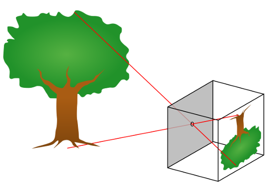The reader is encouraged to try to visualize the effect that changing the focal length $f$ has on the projected image. A perhaps not-so-obvious effect of this projection is that all points along the ray from $O$ to $P$ correspond to the same point $P'$ , as shown below:

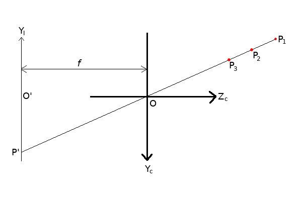
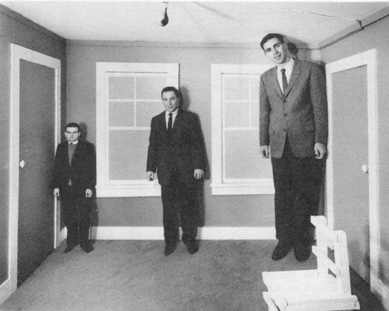
Moving along the $O$ - $P$ ray is equivalent to multiplying both $Y_c$ and $Z_c$ by the same factor, which cancels out when the point gets projected into 2D. This means that depth information is lost under projection, and it’s therefore impossible to recover the original 3D point from our 2D projection without additional information. Humans are able to view a photograph and make sense of distance and proportions because of a magic sauce called context, and it’s why it can be fun to mess with context, like in the Ames room illusion:

Homogeneous coordinates

We will now take a brief mathematical detour in order to introduce the concept of homogeneous coordinates, which will allow us to more easily represent the projection equations as a matrix product. Recall in the previous blog post, when we discussed rigid transformations, we found it useful to augment the coordinates with an additional 1 in order to represent rotation and translation using a single matrix multiplication. This augmentation can be formalized with the theory of homogeneous coordinates and projective geometry, and has applies naturally to the mathematics of projection. Projective geometry is a very rich and deep subject, so we are only covering the bare minimum here in order to proceed. For readers interested in a rigorous but understandable overview in the context of computer vision, Hartley and Zisserman is again a great source.

Homogeneous coordinates can be considered an extension of Euclidian coordinates. For the two-dimensional Euclidian coordinate

$\LARGE \begin{bmatrix} x\\ y \end{bmatrix}$

the corresponding set of homogeneous coordinate are

$\LARGE \begin{bmatrix} zx\\ zy\\ z \end{bmatrix}$

where $z$ is any real number. Thus, each Euclidian coordinate has an infinite number of homogeneous counterparts. For example, $[1, 3, 1]^T$ and $[2, 6, 2]^T$ are both valid homogeneous representations of the Euclidian point $[1, 3]^T$ . In order to recover the Euclidian coordinate, for the homogeneous coordinate $[x, y, w]^T$ one simply normalizes by $w$ to obtain $[x/w, y/w]^T$ .

Whereas Euclidian coordinates live in Euclidian space, homogeneous coordinates live in projective space, where special points with last coordinate 0 are called points at infinity. Projective geometry has all kinds of interesting properties, but for now, it suffices to know the rule for converting from homogeneous to Euclidian coordinates.

The projection matrix

Armed with homogeneous coordinates, we can write our previous projection equations in matrix form, as the following:

$\LARGE \begin{bmatrix}&space;x_I\\&space;y_I\\&space;w&space;\end{bmatrix}&space;=&space;\begin{bmatrix}&space;f&space;&&space;0&space;&&space;0\\&space;0&space;&&space;f&space;&&space;0\\&space;0&space;&&space;0&space;&&space;1&space;\end{bmatrix}&space;\begin{bmatrix}&space;X_c\\&space;Y_c\\&space;Z_c&space;\end{bmatrix}$

where $[x_I y_I w]^T$ are the homogeneous coordinates for $[X_I Y_I]^T$ . Notice that, by simple matrix multiplication, followed by normalization by $w=Z_c$ , we arrive at the same equations for the image coordiates as we did before.

Closing remarks

At the conclusion of this blog, we have learned how to take coordinates in the camera’s frame of reference, and project them onto an image plane. Next, we will perform the final step of scaling the image coordinates into pixels, sum up the model equations and their units, discuss some nonidealities, and end with an example where we write some code to use what we’ve built to solve a simple pose estimation problem.

Part 1: Transformation - here

Part 2: Projection - You’re already here!