If anyone is actually reading these, apologies for not posting this sooner. My work became busier and my baby became a toddler, so my free time has decreased dramatically of late.

Part 3: Scaling

From image to pixel coordinates

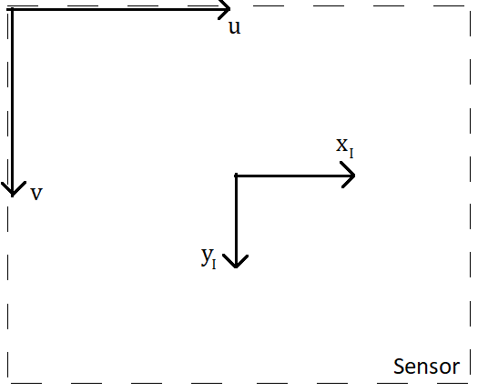
Let’s keep this short, since it’s a pretty simple concept. In the last blog post, we took three-dimensional coordinates in the frame of reference of the camera, and transformed them into two-dimensional coordinates in the frame of reference of the sensor, i.e. what I call “image coordinates”. The last step sends image coordinates, which are in real-world units such as meters, into pixel coordinates, which are in units of pixels. The difference between image and pixel coordinates is shown in the figure below.

The image-to-pixel coordinate transformation needs to first scale the image coordinates into pixel units, and then needs to translate the result so that the origin is at the top left of the sensor. The translation needs to happen because, for computer memory reasons, images are universally indexed so that (0,0) is at the top left. This operation is conveniently written as a matrix multiplication in homogeneous coordinates:

$\LARGE \begin{bmatrix}u\\v\\1\end{bmatrix}=\begin{bmatrix}s_x&0&u_0\\0&s_y&v_0\\0&0&1\end{bmatrix}\begin{bmatrix}x_I\\y_I\\1\end{bmatrix}$

where $u$ and $v$ are the pixel coordinates, $s_x$ and $s_y$ are the scaling factors, and $u_0$ and $v_0$ are added translation terms.

A source of confusion for me was always units, so let’s try to keep the units clear. $x_I$ and $y_I$ are in units of distance, i.e. meters or millimeters, $s_x$ and $s_y$ are in units of pixels per distance, i.e. pixels/m, and $u_0$ and $v_0$ are in units of pixels. So we have a matrix where the units of individual elements are different, which is a consequence of using homogeneous coordinates to represent the transformation.

A brief note on the physical meaning of the values in the scaling and translation matrix: $s_x$ and $s_y$ are almost always equal, and physically represent the horizontal and vertical pixel density of the sensor. To obtain them from a datasheet, you can divide the number of horizontal and vertical pixels by sensor width and height. $u_0$ and $v_0$ are the horizontal and vertical pixel locations of the image center. Usually, these two values will be half of the horizontal and half of the vertical number of pixels, respectively. This is valid for the vast majority of practical applications, but there are some circumstances where the lens isn’t centered with respect to the sensor, like in sensor-shift image stabilization techniques.

However, in nearly all circumstances, the camera’s intrinsic properties (the parameters in the scaling and translation matrix, along with the lens’s focal length) are estimated via a process called camera calibration rather than read off from datasheets. Manufacturing tolerances can mean that what’s on the datasheet isn’t the true value in practice, so calibration is usually performed to obtain the true values, and camera calibration also corrects for lens distortion. I might write a blog post in the future about the basics of camera calibration.

One final practical note: when working with images programmatically, remember that when images are stored in memory as a two-dimensional array, the rows correspond to the y coordinate, and the columns correspond to the x coordinate. Some people (myself included) tend to intuitively think “rows, columns, x, y”, but it’s actually the other way around! Keeping this in mind might save you some pain when going from real-world to pixel coordinates one day.

Putting it all together

Now that we have the final part of our camera model, we can write a single equation which combines all of the transformation matrices, from world coordinates all the way to pixel coordinates:

$\LARGE \begin{bmatrix}u\\v\\w\end{bmatrix}=\begin{bmatrix}s_x&0&u_0\\0&s_y&v_0\\0&0&1\end{bmatrix}\begin{bmatrix}f&0&0\\0&f&0\\0&0&1\end{bmatrix} \begin{bmatrix} r_{11} & r_{12} & r_{13} & t_x\\ r_{21} & r_{22} & r_{23} & t_y \\ r_{31} & r_{32} & r_{33} & t_z \end{bmatrix} \begin{bmatrix} X_w\\ Y_w \\ Z_w \\ 1 \end{bmatrix}$

Note that there is a conversion into non-homogeneous coordinates required for this equation to work ( $u\rightarrow u/w, v \rightarrow v/w$ ). The first and second matrices on the right hand side are often written as a single matrix:

$\LARGE \begin{bmatrix}u\\v\\w\end{bmatrix}=\begin{bmatrix}f_x&0&u_0\\0&f_y&v_0\\0&0&1\end{bmatrix} \begin{bmatrix} r_{11} & r_{12} & r_{13} & t_x\\ r_{21} & r_{22} & r_{23} & t_y \\ r_{31} & r_{32} & r_{33} & t_z \end{bmatrix} \begin{bmatrix} X_w\\ Y_w \\ Z_w \\ 1 \end{bmatrix}$

where $f_x=fs_x$ and $f_x=fs_y$ are the focal length in pixel units. In this way, everything in the matrix has the same units: pixels. The first matrix on the left is called the camera intrinsic matrix, or calibration matrix, and sometimes given the symbol $\mathbf K$ . The second matrix on the left is called the camera extrinsic matrix.

The intrinsic matrix is more generally written with a skew term, i.e.

$\LARGE \mathbf K = \begin{bmatrix}f_x&s&u_0\\0&f_y&v_0\\0&0&1\end{bmatrix}$

where the $s$ has the effect of making $u$ scale with $y_I$ as well as $x_I$ , which introduces a shearing effect to the transformation. However, in all but specific use-cases, the skew term is close to zero.

Conclusion

This completes the projective camera model. I want to finish by mentioning that the projection part of the projective camera model is only one possible projection, for rectilinear lenses. Other types of lenses, for example telecentric, fisheye, or tilt-shift lenses have different projections. The projective camera model, however, is valid for the most common lenses used in photography and machine vision.

Part 1: Transformation - here

Part 2: Projection - here

Part 3: Scaling - You’re already here!

The projective camera model in detail, part three: scaling

Part 3: Scaling

From image to pixel coordinates

Putting it all together

Conclusion