Deep learning for video understanding

This blog aims to give an overview of the history and some of the cutting edge in deep learning for video understanding, with a focus on classification. I’ll try to touch on many different topics in a shallow way, with references to papers at the end if you are interested in reading more. The content in this blog post has been adapted from a talk given to the Vision and AI group at MDA in September of 2020. Let’s get started!

Some of you might already be familiar with various types of deep learning tasks for images. The obvious difference between images and videos is the addition of the time axis, which means

• Removal of motion ambiguity from still frames. Think about a still image taken while a person is in the middle of sitting down. Whereas it’s unclear from a single image whether the person is in the middle of standing up or sitting down, additional frames make the direction of motion obvious.
• An order of magnitude more data per sample. Many modern deep learning video models do some kind of sampling, but even so, a video model must deal with 8 to 32 frames (or more) at once. A typical batch tensor during training for images has four dimensions (Batch, Channel, Height, Width), whereas for videos batches typically have five dimensions (Batch, Channel, Time, Height, Width).
• Models need to deal with video-specific noise, such as compression artifacts, motion blur, and variations of lighting, pose, image quality, etc. between images

So the question is: How can we best leverage and learn from temporal data?

Applications

First and foremost, pretty much every task applicable to images is also applicable to videos. Some popular real-world examples are:

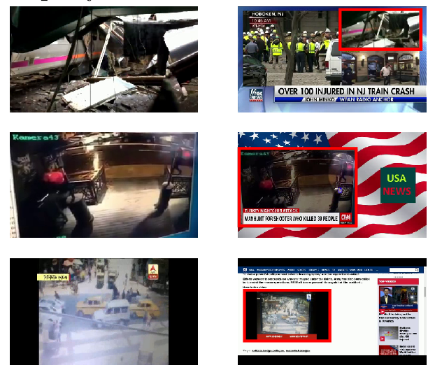
• Banned and copyright content detection
• Anomalous event detection
• Automatic metadata generation and tagging
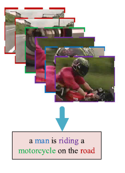
• Automatic video description/captioning (Netflix does this, but with hand-written descriptions)
• Video compression
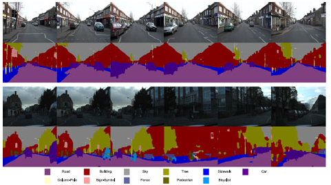
• Scene structuring and parsing, and motion prediction (e.g. for self-driving cars)

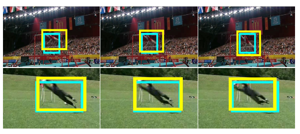
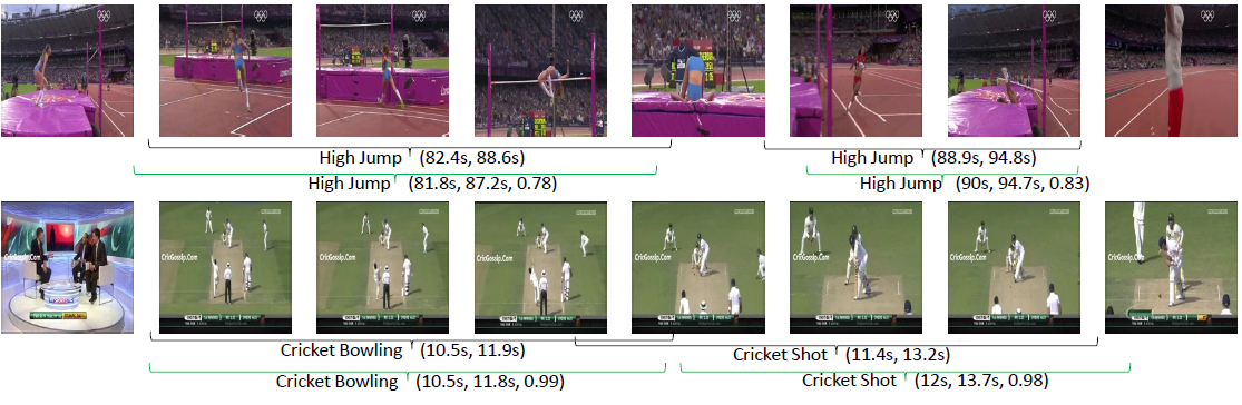
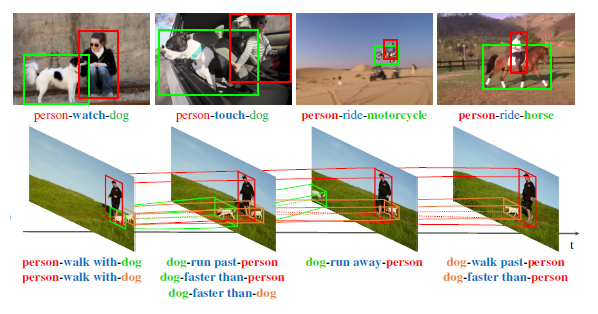
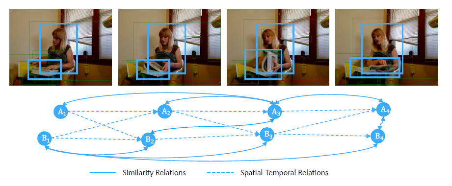
Also, here are some specific machine learning tasks from the literature:

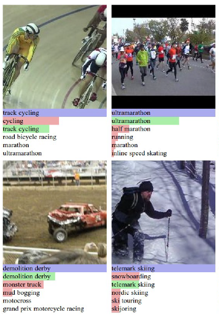
In this blog, we will focus on video classification, and give an overview of the history, current architectures, and challenges pertaining to video classification via deep learning. Classification tends to be the most important task to track progress in a field because:

• classification architectures tend to improve first and fastest,
• improvements in classification can be thought of as improvements in feature extraction and representation learning,
• classification architectures, weights, and features are frequently used as backbones for other tasks.

We will specifically discuss 3D convnets, which give state-of-the-art results as of 2020.

Timeline

Pre-2014

Before 2014 means before the explosion of deep learning in computer vision. At this time, most vision tasks were performed with hand-crafted features plugged into either a hand-crafted classifier or a shallow machine learning classifier (i.e. an SVM or logistic regression). The state-of-the-art before the deep learning era was improved dense trajectories (iDT).

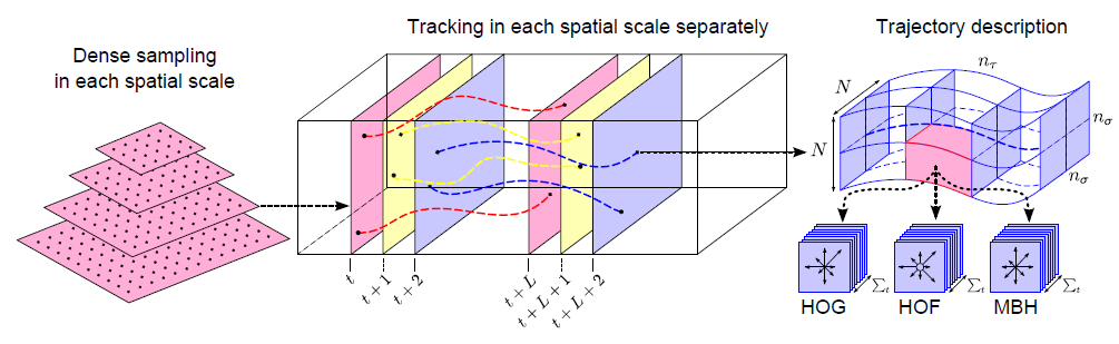
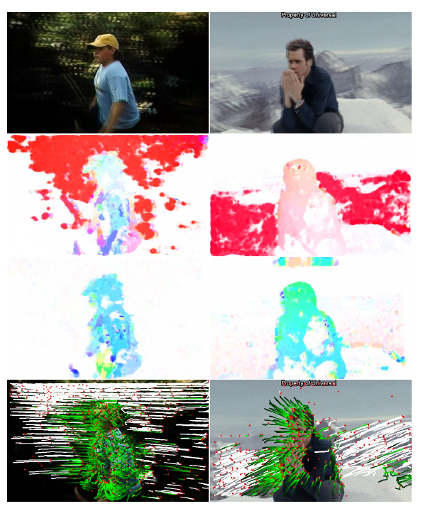
iDT computed HoG (histogram of oriented gradient) features from individual images and HoF (histogram of optical flow) and MBH (motion boundary histograms) features from dense optical flow, repeated for different scales, did some processing, stacked things together, and passed the resulting feature vector into an SVM for classification.

iDT did what a lot of vision classifiers did before deep learning: find a clever way of extracting and packaging hand-crafted features, and train a classifier to make predictions using them. iDT actually performed very well on what is still a difficult problem, but it had some issues which would later be solved by deep learning:

1. iDT only contained low-level features, rather than the much richer semantic features that we can now get from deep neural networks
2. Dense optical flow was (and still is) expensive, especially for real-time applications
3. Dense optical flow is sensitive to camera motion and scene changes

2014

2014 represents the start of the use of deep learning in video classification. Two architectures are representative of this period.

The two-stream 2D convnet is an architecture where two separate convnets are used to extract features, one from still images, and the other from optical flow.

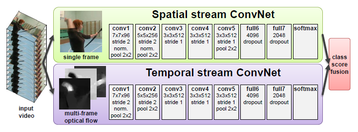
In Simonyan’s network, one convnet branch takes a randomly sampled RGB frame, and the other branch takes a stack of dense optical flow frames. In the original work, the RGB network is pretrained on ImageNet, whereas the optical flow network is trained from scratch. Finally, the class logits from the two networks are averaged to make predictions. Most notably, the optical flow frames are stacked along the channel dimension, and not a fifth time dimension, making both streams 2D convnets rather than 3D convnets.

This idea of using both images and optical flow was seen with iDT, and is a feature of multiple other architectures, most notably I3D, which we will go into detail about later. Generally, adding dense optical flow as features improves accuracy by a few percent, but makes prediction much more computationally expensive.

DeepVideo was a network that used RGB frames as inputs only, but experimented on different ways of “fusing” the features from frames.

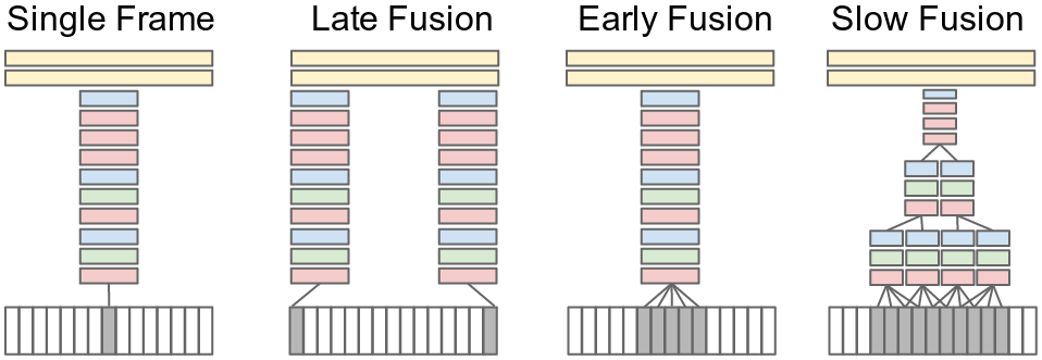
Late fusion concatenated 2D convnet features from two frames far apart, whereas early and slow fusion used 3D convnets to extract features from a temporally-stacked set of frames. Unsurprisingly, slow fusion was found to be the best performing, and this work by Karpathy was the start of the rise of 3D convnets.

2015

LCRN uses what seems like an obvious idea: videos are sequences of images, so why not use a sequence-prediction model? LCRN passes images into a 2D CNN, whose output features are sent into an LSTM. The LSTM could then be used for sequence-to-sequence or sequence-to-fixed preditions.

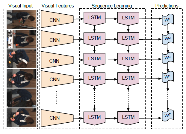
LCRN’s architecture is, in fact, identical to early image captioning models, except that a sequence of images is sent to the LSTM instead of a single image with different attention masks. The problem was that low-level features tended to get “lost” in the CNN-to-LSTM structure, which typically only retained abstract features.

C3D was the first widely cited fully 3D convolutional neural network on videos, and was, at the time, the best performing model on a number of video datasets. C3D featured 3x3x3 convolutional kernels, and 3D pooling layers, for a completely model until the final fully-connected layers. C3D was interesting both for its high performance, and its simplicity: it performed well with just an Alexnet-style CNN, without the LSTMs and multiple branches of its predecessors.

After the success of C3D, it became clear that 3D convnets were better-performing than 2D convnets on videos, and a search for improved architectures began. This takes us to an important aside: Why is 3D convolution along a time axis better than 2D convolution on channel-wise stacked images?

The answer is straightforward: 3D convolution is better able to capture and preserve temporal information, which is said to “collapse” when applying 2D convolutions only. The other reason is that weight sharing means that the weights for 3D convolutional layers can be reused when applied to multiple successive frame segments. These are exactly the same reasons why 2D convolutional layers are used for images instead of fully-connected layers.

2017

I3D is a 2-stream 3D convnet, similar in concept to earlier two-stream networks, except that both branches are 3D convolutional networks. Like earlier networks, one branch takes a stack of frames, while the other takes a stack of dense optical flow, with logits averaged between the two branches at the output. Each branch of the network was trained separately, and averaging predictions again gave a few percent better accuracy than either of the two branches individually.

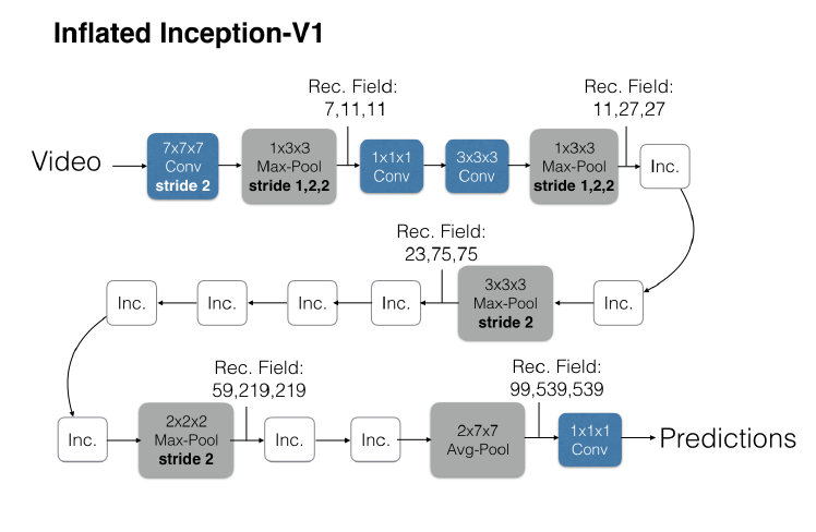
One key advancement of I3D was to base its layers on the well-known Inception (v1) architecture, and then “inflate” Inception’s weights so that starting weights came from the pretrained image classification network. This inflation is simple: just make each filter in a 3D convolutional layer have the same weights as the filter in the 2D convolutional Inception layer (after normalization across time). This way, a video where all of the frames are identical gets layer-by-layer output activations which are identical (after averaging across time) to Inception. Another tiny implementation detail is that I3D used a single long stack of frames – over 80 – to make predictions whereas nearly all other modern networks sample multiple shorter stacks – 8 to 32 frames each – and average their predictions during inference.

R3D are 3D Resnets. Resnets, of course, had been around for a few years by the time this paper was published, but it had taken some years for video models (which are a less popular area of research) to catch up to the latest advancements in image classification. R3D had all of the essential features of Resnets: a stack of standard layers which successively pool down space while increasing the number of channels, and residual connections across layers.

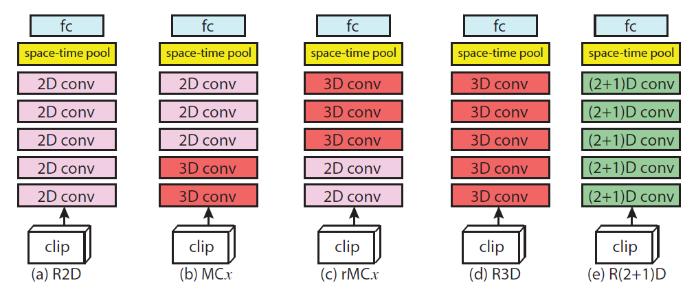
A major contribution of R3D was the introduction of the factorized R(2+1)D layer, which is a 1xdxd spatial-only filter followed by a tx1x1 time-only filter, reducing the number of weights compared to a single txdxd filter:

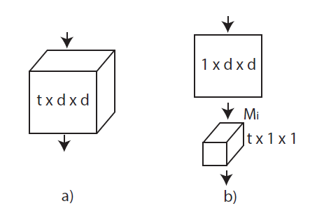
The idea of decomposing convolutional layers into parts had been explored earlier in image models, and this was another case of video models taking inspiration from the larger body of research available on image understanding. Experimentally, when the R(2+1)D network and the fully 3D Resnet had the same number of weights, the R(2+1)D network was found to have superior performance.

2019-present

At this point, we are in an era where people are tweaking the general formula of 3D Resnets, either architecturally, with augmentations, regularization, or frame sampling. Here are two examples. Both of the networks summarized here performed at the state of the art when they were published.

As an aside, all modern networks now use the strategy of sampling multiple small frame segments, and averaging their inference outputs. When compared to the strategy of using a single long segment, this avoids the implementation problem of sometimes needing to loop or pad frames for short videos.

SFN, or Slow-Fast networks, are two-branch 3D Resnet(-101) networks, except that instead of having branches for RGB and optical flow, SFN’s branches sample RGB frames at different strides.

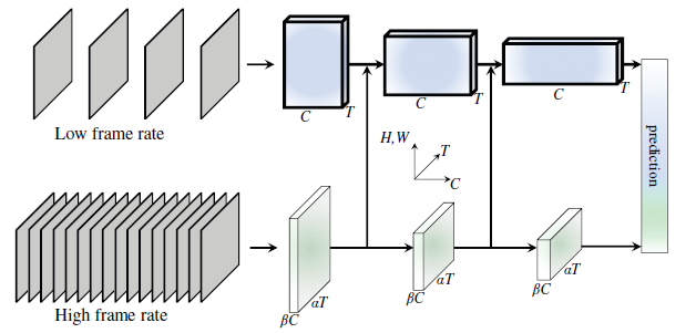
The slow branch samples every 8 or 16 frames, and the fast branch samples every 2 frames. The authors suggest that spatial features are learned in the slow branch, whereas temporal features are learned in the fast branch. At train time, a short (16 frame) clip is randomly sampled from the video, whereas at inference time, 10 random clips with 3 different spatial crops (30 stacks total) are sent through the network with averaged logits at the output.

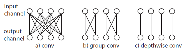
CSN, or Channel-separated 3D networks, are 3D resnets which have their convolution layers decomposed into 1x1x1 full-channel convolutions, and 3x3x3 grouped single channel convolutions. In other words, these are essentially fully connected layers on a single pixel of a 3D feature map, and regular convolutional kernels on a single channel, respectively.

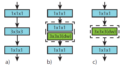
The effect of these channel-wise decompositions is significant: the network is easier to train, less expensive to perform inference, and channel separation is also thought to have a regularizing effect. CSN performed at the state of the art at time of publication, and outperformed R3D and R(2+1)D with less computational cost.

Modern video classification

Challenges and directions for future work

The main problems in the field are the lack of large, general, labeled video datasets, as well as the high disk, memory, and processor requirements to train on video datasets. Datasets have historically been small, and focused on human actions (sports, everyday interactions, etc.). Some historical examples are:

• HMBD-51 [Kuehne, 2011]: 51 human action classes, around 7,000 clips
• UCF101 [Soomro, 2012]: 101 human action classes, around 13,000 clips
• ActivityNet [Heilbron, 2015]: 200 human action classes, around 28,000 clips
• Kinetics-400 (and -600, -700) [Kay, 2017]: 400 human-object and human-human interaction classes, around 300,000 clips

Given the additional variance introduced by the time axis and the large representational capacity of 3D convnets, training on smaller datasets is incredibly prone to overfitting. Much of the accuracy of modern image models comes from pretraining from ImageNet and other huge datasets, but this type of extremely general, vast dataset is simply not available for videos. The best that video models can do currently is bootstrap their weights from ImageNet-trained 2D networks, and then pretrain on Kinetics-400, Kinetics-600, or Kinetics-700.

Video augmentation

One area of active research for video models is augmentation. Augmentation for images has been thoroughly explored, and frameworks such as imgaug and torchvision allow easy construction of powerful image augmentation pipelines. Similar frameworks (as of 2020) don’t really exist for videos.

Additionally, due to the addition of the time dimension, a number of possibilties exist for video augmentations that didn’t exist for images. First, all image augmentations can be applied to videos, in a number of ways. For example, augmentations with a parameter (like rotation) can have the parameter vary randomly, smoothly, or uniformly through time.

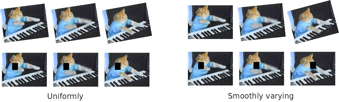
There are also augmentations unique to video, where frames are messed with in various ways:

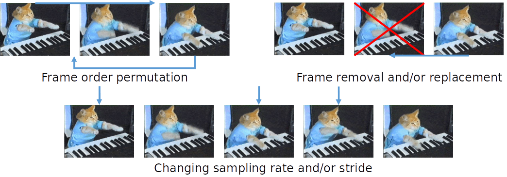
Overall, stronger augmentations can help with regularization and overfitting, which is a big problem for video understanding.

Semi-supervised and self-supervised learning

Image classification models have undergone (relatively) large leaps in performance by leveraging unlabeled data, as well as so-called “weakly-labeled” (noisy or differently-labeled) data. The same gains in performance can be made for video models, especially considering the huge amount of unlabeled and noisily-labeled videos being generated every second on the internet.

Ideas like consistency regularization, pseudo-labeling, and entropy minimization have all generated a lot of research interest in recent years. On the deep learning side, there is also the idea of using pretext tasks to learn representations as a form of pre-training. With the proper engineering and implementation, any of these have the potential to dramatically boost performance in video understanding.

References

• [Karpathy, 2014] Karpathy, Andrej, et al. “Large-scale video classification with convolutional neural networks.” Proceedings of the IEEE conference on Computer Vision and Pattern Recognition. 2014.
• [Gao, 2017] Gao, Lianli, et al. “Video captioning with attention-based LSTM and semantic consistency.” IEEE Transactions on Multimedia 19.9 (2017): 2045-2055.
• [Zhou, 2018] Zhou, Bolei, et al. “Temporal relational reasoning in videos.” Proceedings of the European Conference on Computer Vision (ECCV). 2018.
• [Kalogeiton, 2017] Kalogeiton, Vicky, et al. “Action tubelet detector for spatio-temporal action localization.” Proceedings of the IEEE International Conference on Computer Vision. 2017.
• [Qiu, 2017] Qiu, Zhaofan, Ting Yao, and Tao Mei. “Learning deep spatio-temporal dependence for semantic video segmentation.” IEEE Transactions on Multimedia 20.4 (2017): 939-949.
• [Kordopatis-Zilos, 2019] Kordopatis-Zilos, Giorgos, et al. “Visil: Fine-grained spatio-temporal video similarity learning.” Proceedings of the IEEE International Conference on Computer Vision. 2019.
• [Shang, 2017] Shang, Xindi, et al. “Video visual relation detection.” Proceedings of the 25th ACM international conference on Multimedia. 2017.
• [Wang, 2018] Wang, Xiaolong, and Abhinav Gupta. “Videos as space-time region graphs.” Proceedings of the European conference on computer vision (ECCV). 2018.
• [Wang, J. Comp. Vis. 2013] Wang, Heng, et al. “Dense trajectories and motion boundary descriptors for action recognition.” International journal of computer vision 103.1 (2013): 60-79.
• [Wang, ICCV 2013] Wang, Heng, and Cordelia Schmid. “Action recognition with improved trajectories.” Proceedings of the IEEE international conference on computer vision. 2013.
• [Simonyan, 2014] Simonyan, Karen, and Andrew Zisserman. “Two-stream convolutional networks for action recognition in videos.” Advances in neural information processing systems. 2014.
• [Tran, 2015] Tran, Du, et al. “Learning spatiotemporal features with 3d convolutional networks.” Proceedings of the IEEE international conference on computer vision. 2015.
• [Donahue, 2015] Donahue, Jeffrey, et al. “Long-term recurrent convolutional networks for visual recognition and description.” Proceedings of the IEEE conference on computer vision and pattern recognition. 2015.
• [Carreira, 2017] Carreira, Joao, and Andrew Zisserman. “Quo vadis, action recognition? a new model and the kinetics dataset.” proceedings of the IEEE Conference on Computer Vision and Pattern Recognition. 2017.
• [Tran, 2017] Tran, Du, et al. “A closer look at spatiotemporal convolutions for action recognition.” Proceedings of the IEEE conference on Computer Vision and Pattern Recognition. 2018.
• [Feichtenhofer, 2019] Feichtenhofer, Christoph, et al. “Slowfast networks for video recognition.” Proceedings of the IEEE international conference on computer vision. 2019.
• [Kuehne, 2011] Kuehne, Hildegard, et al. “HMDB: a large video database for human motion recognition.” 2011 International Conference on Computer Vision. IEEE, 2011.
• [Soomro, 2012] Soomro, Khurram, Amir Roshan Zamir, and Mubarak Shah. “UCF101: A dataset of 101 human actions classes from videos in the wild.” arXiv preprint arXiv:1212.0402 (2012).
• [Heilbron, 2015] Caba Heilbron, Fabian, et al. “Activitynet: A large-scale video benchmark for human activity understanding.” Proceedings of the ieee conference on computer vision and pattern recognition. 2015.
• [Kay, 2017] Kay, Will, et al. “The kinetics human action video dataset.” arXiv preprint arXiv:1705.06950 (2017).
• [Tran, 2019] Tran, Du, et al. “Video classification with channel-separated convolutional networks.” Proceedings of the IEEE International Conference on Computer Vision. 2019.
• [Gidaris, 2020] Gidaris, Spyros, Praveer Singh, and Nikos Komodakis. “Unsupervised representation learning by predicting image rotations.” arXiv preprint arXiv:1803.07728 (2018).
• [Chen, 2020] Chen, Ting, et al. “A simple framework for contrastive learning of visual representations.” arXiv preprint arXiv:2002.05709 (2020).